
![]()
| |
|
|
|
|
Intusoft
Newsletter Issue #52, February 1998
Copyright
©2002 Intusoft, All Rights Reserved
| In This Issue | |||
|
1 10 12 16 |
18 18 19 |
||
In this article, we lay out a method for test synthesis that is is based upon standards which have been developed for the aerospace industry. Like VHDL in the past, affordable tools are available to migrate this technology to the commercial sector. Benefits of this migration include improved production quality, a reduction in the quantity of spare parts, and dramatically improved time to market. For today’s competitive aerospace companies, these techniques are a necessity!
|
How Should A Circuit Be Tested?
Traditionally, the designer specifies test requirements which verify proper functionality of his creation. Frequently, these requirements are just a pass-through of the product specification. Many contemporary designs are fault tolerant; they may meet their functional specification even if they contain failed or out-of-tolerance parts. Testing only to functional requirements may allow a product to ship with one or more failed components. While these failures may not impair its functionality, as measured by the acceptance test, they increase the odds that the product will fail shortly thereafter. To remedy this situation, the test engineer or the circuit designer may want to expand the functional test requirements in order to find these component failures. The objective of this "test synthesis" is to define a set of tests that;
a) makes sure that the product works when delivered,
b) rejects a Unit Under Test (UUT) that has failed parts,and
c) enumerates the failures.
Overlaying these objectives is the dual desire not to cause any damage to the UUT through testing, and to perform efficient tests which have robust conclusions. Efficiency minimizes the number of tests that are needed in order to reach a conclusion. Robust testing requires the minimization of false test results.
|
What is a Failure?
A good design can accept part tolerances that are far wider than the tolerances of the individual components. For example, a 2kW pull-up resistor could work just as well as the specified 1kW resistor. Clearly, we want to accept the out-of-tolerance part in order to take advantage of the increased yield provided by a robust design. Production engineers should be able to substitute parts based on cost and availability. In the resistor example described above, an open pull-up resistor could actually pass a functional test, and fail in the next assembly when the noise environment increases. It is reasonable to conclude that we want to detect and reject products which have catastrophic component failures; but we can accept products which have parametric "failures" that do not affect functional performance. Actually, these parametric failures are part of the tolerance distribution of the parts we are using. Monte Carlo analysis will indicate the robustness of the design when we compare the resulting performance predic-tions with the product specification.
Defining Failure Modes
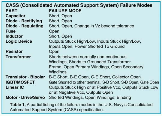
Component failures are well characterized by a finite number of catastrophic failure modes. For digital circuits, there are 2 failure modes; stuck at logic one and stuck at logic zero. Film and composition resistors are characterized by open circuit failures. Table 1 is the way the US Navy characterizes the catastrophic failures for many common parts. You may define failure modes using common-sense experience, historical data or physical analysis. Depending on your application, you might want to consider additional failures; for example, bridging or interconnect failures in ICs that result in shorts between de-vices. In a PCB design, you might want to simulate high resistance "finger print - shorts" caused by improper handling of sensitive components. Abstracting subassembly failure modes to the next assembly is a common error. Consider the case of an IC op-amp. The failures detected and rejected by the op-amp foundry are mostly caused by silicon defects. Once eliminated, these defects will not reappear. At the next assembly, failures are caused by electrical stress from static electricity, operator error in component testing, or environmental stress in manufacturing. This requires defining a new set of failure modes at the next production level. Again, we can usually describe these failure modes using catastrophic events at the device or assembly interface; that is, open, short or stuck for each interface connection.
Unusual Failure Modes are Infrequent
Unusual failure modes get a lot of attention; for example, finding a PNP transistor die in an NPN JANTXV package. Although these things do happen, they are very rare. If acceptance testing detects only 99% of failed parts, then the quality of your product increases 100 fold after these tests are performed. For many products, that increased quality means there will be no undetected failures delivered to the customer.
Detecting Process Faults
Process faults could cause the shift of many parameters simultaneously. When this is a consideration (usually for ICs), the process parameters are monitored separately. If the process fails, the unit is rejected before the acceptance test is performed. Therefore, acceptance testing does not need to account for multiple parametric fault modes.
What’s A Test?
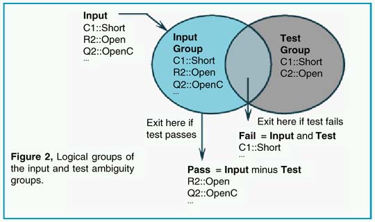
In order to compare one test with another, there must be a precise definition of the test. A test is defined as the comparison of a measured value with its test limits. The result of the comparison leads to the conclusion that the UUT either passed the test or failed the test. At the beginning of the test, there is a set of failure modes that have not been tested; these are defined by the Input Ambiguity Group. The test itself is capable of detecting a number of failure modes. These modes are grouped into a set called the Test Ambiguity Group. The pass and fail outcomes then carry a set of failure modes which are the result of logical operations carried out between the Input Ambiguity Group and the Test Ambiguity Group such that:
|
where AND represents the intersection of the lists, and MINUS removes the elements of one group from the other. Using MINUS here is a convenient way of avoiding the definition of NOT (Input…), since we really aren’t interested in a universe that’s greater than the union of the Input and Test ambiguity groups. Figure 2 illustrates this logic. The fail or pass outcomes can then be the input for further tests. If further tests are only connected to the pass output, then a product acceptance test is created. If tests are connected to both the pass and fail outcomes, then a fault tree is created; the fault tree isolates faults for failed products. In either case, the object of each test is to reduce the size of the pass ambiguity group. When the addition of more tests can’t further reduce each pass ambiguity group size, the test design is considered to be be completed. It turns out that characterizing the "no fault" case as a member of the initial ambiguity group, or failure universe, will be useful later on when we decide which test is the best.
Selecting The Best Test
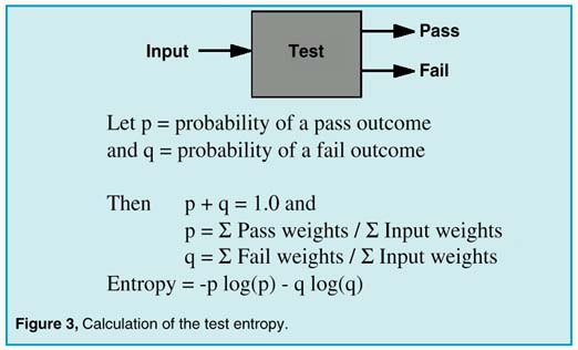
A terminal conclusion is defined as the pass or fail conclusion for which no more tests can be found. Then, if the no fault mode is present, it is the product acceptance test result, with all remaining faults being the ones that are undetectable. Other wise, the parts with the resulting failure modes are the set that would be replaced in order to repair the UUT. In general, our goal is to reach the terminal pass/fail conclusions by performing as few tests as possible to reach each conclusion. The general solution to this problem using an exhaustive search technique expands too rapidly to find a solution during the lifetime of our universe… it’s an N-P complete problem. Several heuristic approaches are possible, one of which follows. If we take the idea of failure modes one step further, we can give each failure mode a failure weight that is proportional to the failure rate. To avoid looking up failure rates, we can default these weights to 1.0, and later we can assign a more precise value. The weights will be used to prioritize the search for the best test, and weighting the test that isolates the parts with higher failure rates first. For each test candidate, we can compute the probability of a pass outcome and a fail outcome. From a local point of view, the summation of the pass and fail probabilities must be unity; that is, the UUT either passes or fails a particular test. Borrowing from information theory, we can compute the test entropy as shown in Figure 3:
|
The highest entropy test contains the most information. We select the best test as the test which has the highest entropy. For the case when failure weights are defaulted to unity, this method will tend to divide the number of input failures into 2 equal groups. Since "no fault" can only be in the pass group, a high "no fault" weight will steer the tests through the pass leg fastest, making the best product acceptance test. The rationale for a high "no fault" probability is the expectation that most units will pass the production acceptance test; this is a condition of an efficient and profitable business. If, on the other hand, we want to test a product that was broken, we would give the "no fault" probability a lower value. Then the test tree would be different, having a tendency to isolate faults with fewer tests.
Test Sequencing
The definition of the best test did not include the difficulty of setting up the test or performing it; and it didn’t include the potential of a failed part to destroy other parts. In addition, the tests were selected independent of the product specification so that we could get to the terminal pass outcome with a tolerance failure. To overcome these problems, tests are sequenced. The sequence priority is:
1. Perform tests that eliminate failure modes that could be destructive in future tests. Frequently, this requires a new test configuration that performs a "safe to start" test.
2. Perform easy tests first, such as DC measurements at room temperature.
3. Perform similar tests in sequence, such as rise time tests which use the same test equipment.
4. Repeat the process for major setup changes, such as measurements under high temperature conditions.
What About Required Tests?
We will discuss robust testing next, however, if we take a hypothetical product specification, we can see that faults will usually show up with wider test limits than the product specification limits. These tighter limits make it possible for tolerance failures to appear as catastrophic failures. If we do fault isola-tion, the wrong conclusion could be reached. Basically, the required tests need to be placed in as harmless a place as possible, usually at the end of the sequence in which they are found. Functional limits should not be used for fault isolation unless they are also robust.
Tolerances can cause measurement results to migrate across the test limit boundary. As a result, a fault could be classified as good, or a good part could be classified as a failure. Tolerances include:
· UUT part tolerances
· computer model accuracy
· measurement tolerances
· UUT noise
· test set noise
· fault prediction accuracy
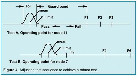
Avoiding false test conclusions requires setting the test limits as far away from the expected results as possible. To compare one test with another, we need to define a measure of test robustness. A test measurement, for a UUT that is good, has a range of values (called a "tolerance band") that defines acceptable performance. The measure of test robustness with respect to a failure mode is then the distance between the failed measurement result and the nearest test limit, divided by the tolerance band. We call this value a "guard band". The test limit can be safely placed in the guard band as long as no other faults have results in this band. Normalizing all measurements using their tolerance band allows us to compare the guard bands of different tests. We can then modify the entropy selection method to reject tests which have small guard bands. Figures 4 and 5 show how this works.
|
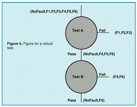
In this example, we have 2 operating point tests. Failure modes are identified as NoFault, F1, F2, …F6. It is assumed that test A is performed first, and test B is performed on the pass group of test A, as shown in Figure 5. Test A divides the failures into a pass group containing F4,F5,F6 and a fail group containing F1,F2,F3. Connecting test B to the test A pass outcome eliminates F1 from the test B failure input. The guard band for test B extends from the hi limit to F4. If test B were done first, the guard band would be smaller, from the test B hi limit to F1.
|
An incorrect test outcome will invalidate subsequent test decisions. In order to be correct most often, tests with large guard bands should be performed first, since they are less likely to be incorrect. Moreover, tests that were previously rejected may turn out to be excellent tests later in the sequence, as illustrated in the example. Tests with small guard bands simply should not be used. While a model of the statistical distribution is shown in Figure 4, you should be aware that there usually isn’t sufficient information to have a complete knowledge of the statistics of a measurement result. In particular, the mean is frequently offset because of model errors; for example, a circuit that is operating from different power supply voltages than was expected. The statistics of failed measurements are even less certain because the failure modes and the failed circuit states are less accurately predicted. It is necessary, therefore, to increase the tolerance band as much as possible. We avoided stating exactly where in the guard band the measurement limit should be placed; it’s a judgment call, depending on how much the tolerance band was widened, and on the quality of the fault predication.
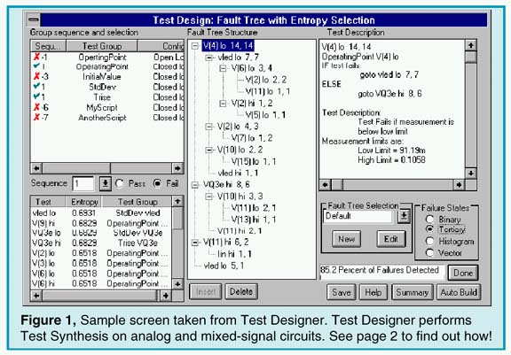
Conclusion
Testing can extend well beyond the traditional functional performance demonstrations of the past. Now you can synthesize tests for analog and mixed-signal circuits and guarantee a fault coverage percentage, just like you do for your digital tests. Moreover, faults can be isolated to facilitate repair or enhance quality management. Dramatic improvements in EDA software (for example, our Test Designer product - see Figure 1) has enabled these comprehensive test development features to be included in any design, and at a reasonable cost. You can visit our web site at www.intusoft.com and download a detailed brochure, application notes, and an evaluation version of Test Designer, or email us at test@intusoft.com to arrange for a personal on-site demonstration.
[1] CASS Red Team Package data item DI-ATTS-80285B, Fig. 1 - SRA/SRU Fault Accountability Matrix Table.
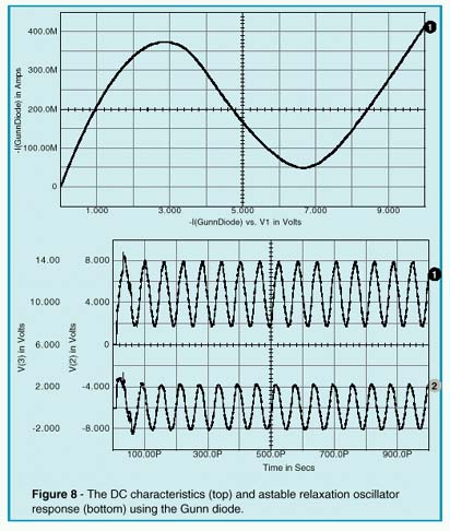
A GUNN DIODE RELAXATION OSCILLATOR
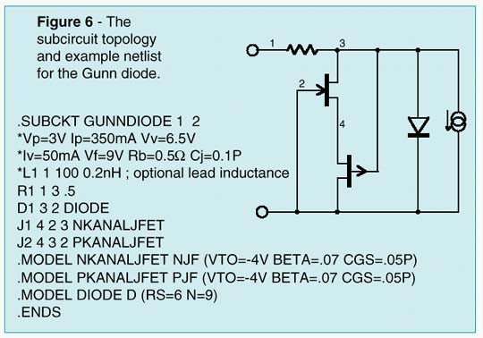
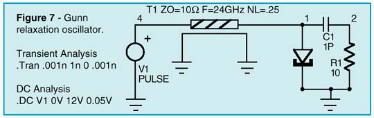
Transferred Electron Devices (TEDs), widely know as Gunn diodes, are gallium arsenide (GaAs) or indium phosphide (InP) devices which are capable of converting direct current (DC) power into radio frequency (RF) power when they are coupled to the appropriate resonator. Typical applications for Gunn diode oscillators include local oscillators, voltage controlled oscillators (VCOs), radar and communication transmitters, Doppler motion detectors, intrusion alarms, police radar detectors, smart munitions, and Automotive Forward Looking Radars (AFLRs). Gunn Diodes are two-terminal negative-impedance semi-conductors which are similiar to tunnel diodes (See Intusoft Newsletter 51, Nov. 1997). They are mainly found in micro-wave oscillators in the range from ten to several hundred Gigahertz. The negative differential impedance of the Gunn diode may be modeled by a complementary pair of JFETs, as shown in Figure 6. In Figure 7, an example Gunn relaxation oscillator is shown. Three criteria must be met in order for this circuit to operate properly. First, the DC source resistance must be less than the negative impedance. Second, the load-line must intersect the active characteristic in the negative impedance region. Third, the AC impedance of the DC source must be very high in order to ensure that the bias point becomes astable. The first and last conditions can be met by the
|
|
transforming properties of a quarter-wavelength transmission line. Oscillation occurs at that repetition frequency (see Figure 8) due to the fact that the zero impedance of the DC source appears infinitely high at the gunn diode.
[1] Litton Solid State Division Applications Notes InP and GaAs Gunn Diode Devices, June, 1997.
|
FMCW-DISTANCE RADAR
by Karl Heinz Muller
For more than 40 years, Radar Altimeters have been used in avionics to measure the altitude of airplanes over ground. Advanced developments of Gallium Arsenide millimeter-wave chips have lead to a considerable reduction in costs, thereby allowing this technique to find more and more acceptance with earthbound traffic control systems. After the invention of the air bag and anti-blocking systems, the automotive radar is poised to become the third significant part of this genre of safety equipment.
A Radar Sensor for Advanced Cruise Control
The ideal cruise control would be one that could measure the distance between vehicles and adjust it, depending on the general traffic speed. In order to accomplish this, a self-contained sensor must be mounted on the vehicle. With a vehicle-mounted radar, it is possible to:
· Measure the position and speed of all objects in front
· Ignore all irrelevant objects (e.g. crash barriers, approach-ing traffic)
· Distinguish between vehicles in different lanes
· Lock-on to the closest vehicle in the same lane
· Continuously output Range, Speed and Angle for the locked-on vehicle
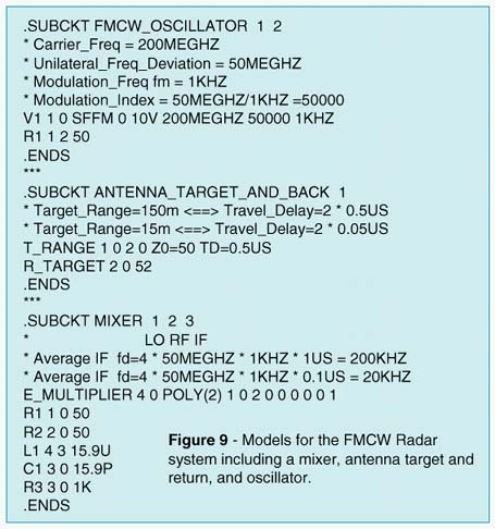
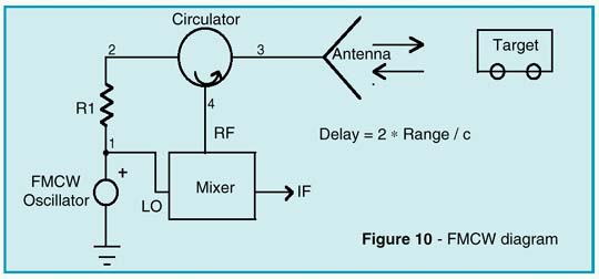
Frequency-Modulated-Continuous-Wave (FMCW) radar has many applications. In FMCW applications, the distance mea-surement is derived by a transmitter/receiver combination that is continuously and linearly swept from a low frequency to a high frequency. FMCW radar is based upon on the doppler effect. For example, if the lower and upper frequencies are 2000MHz and 5000MHz, and a 2000MHz signal is transmitted and hits an object, a reflection is received from that object to the antenna. By the time the signal reaches the antenna, the transmitted signal would have been, for example, 2005MHz. The returning signal at 2000MHz and the transmitted signal at 2005MHz are fed into the mixer, yielding an intermediate frequency of 5MHz. The intermediate frequency is directly proportional to the distance to the reflecting surface. The FMCW-distance radar (see Figure 10) is intended for collision avoidance and cruise control on heavily loaded high-ways. Due to the high speed of electromagnetic propagation, an unmodulated high frequency carrier alone is not suited to
|
detect a travel delay of a received waveform caused by reflections from a distant target. With pulse modulated carriers, for example, the leading edges of the leaving and returning pulses can be utilized for this purpose. As an alternative, FMCW systems use the instantaneous carrier frequency shift between the transmitted and received signal to measure the delay, td=2r/c, which is proportional to the distance, r. This is accom-plished via a mixer which operates as a multiplier for both signals, by generating sum and difference frequencies. While the sum is suppressed by a low pass filter, the difference appearing at the IF port is used for further signal processing.
|
|
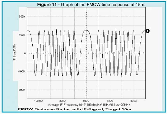
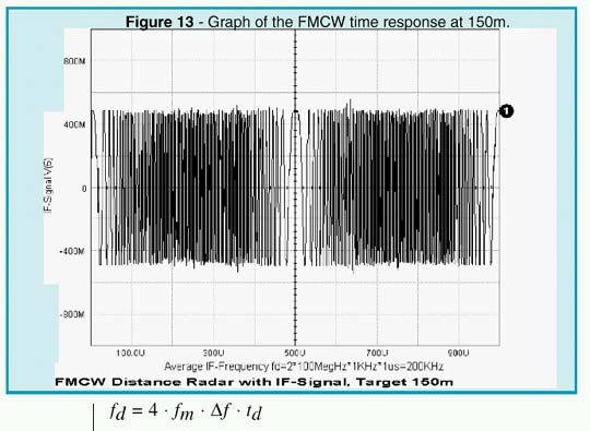
A circulator can be used to separate the transmitting and receiving paths. Therefore, only a single antenna is needed for both channels. Modeling of the distance and reflecting cross section of the target is realized by a slightly mismatched bidirectional delay line. Depending on the standing wave ratio, or reflection coefficient, only a small fraction of the transmitted power is reflected and appears at the RF port of the mixer. As shown by the simulation (Figures 11 and 13), the intermediate frequency is proportional to the distance of the target.
The average frequency may be calculated by the equation:
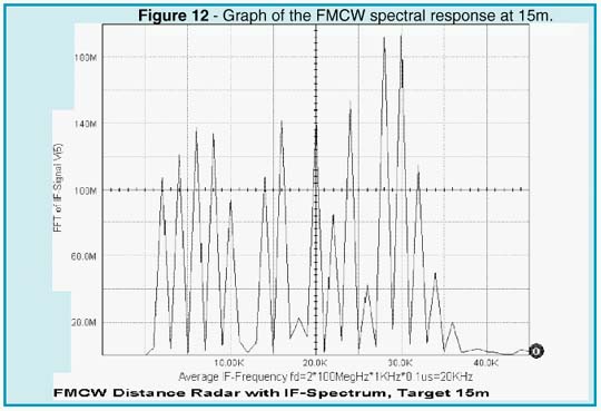
|
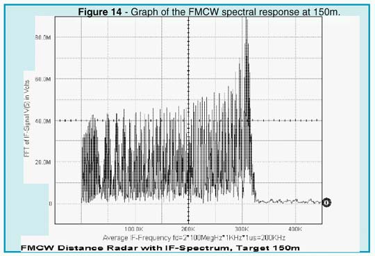
|
The result depends upon the modulation frequency, the unilateral carrier frequency deviation, and the total travel delay time. A more detailed Fourier analysis (see Figures 12 and 14) reveals that the total IF spectrum consists of integer multiples of the modulation frequency whose amplitudes follow the Bessel function. The averaging process may simply be done by a counter that is gated by the modulation period (1/fm). By selecting proper scaling, the counter then displays the true distance of the target.
|
Will Your Vendor Supply These Features???
Is Your Specialty Supported?
Analog - Mixed Signal - Power - RF - System - Test - FMEA
It's time to turn to Intusoft for proven technology from a stable company that you can count on. Intusoft has a reputation for placing state-of-the-art technology on your desktop and providing you with the support and training needed to make your job easier, faster, and more productive. Unlike other companies, we don't force you into a single solution. You can integrate our simulation suite with 3rd party schematics, or use our advanced configurable schematic tool to drive your design.
For a Limited Time Offer...
PSpice Users can turn to Intusoft now; by simply purchasing a maintenence and a training class, you will receive a full ICAP/4 package, along with a 30% discount on most other Intusoft products. Call Intusoft for details or email : help@intusoft.com
Much ado has been made of the year 2000 calendar problem for computers. For the most part, the problem exists for legacy software that compares dates using the last 2 digits of the calendar year; Intusoft software doesn’t do this. Intusoft uses dates only for printing on reports and checking file status. Sample IsSpice4 banner :
******* Fri Jan 02 08:59:50 ******* IsSpice4 ver. 7.6.4 ******* 8/15/98
We assume the user will know whether his simulation took place in the year 1900 or the year 2000, so unless there is a strong user sentiment to change the year to 4 digits, we plan no change in this output format. After all, if people can recognize the year, so should computers. The time application interface that we use counts time in seconds, beginning in the year 1970. It uses a signed long variable to hold the value - it can hold up to 68.1 years in seconds; the end of time will occur in the year 2038, at least for this method of counting. Long before this happens, we expect to switch over to 64 bit systems, so the problem will simply vanish as the technology matures.
Newsletters Page | Issue 54 | Issue 53 | Issue 52 | Issue 51 | Issue 50
©2002 Copyright Intusoft, All Rights Reserved.