
|
|
|
Downloads and Links Microchip Solar2TiM Eval Board
|
DSP Designer is used for development of control systems implemented using digital signal processors. There are 5 components:
The optional hardware
evaluation kit is designed to get you started with a real-world design.
|
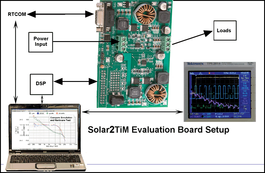
Hardware Option
The hardware option
includes 1 Intusoft Solar2TiM dual synchronous buck/boost PWM regulator
with connectors that accept either of the above DSP evaluation kits. |
 |
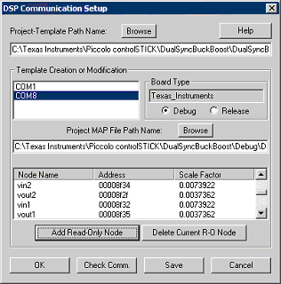
Real time communication
uses a small footprint DSP based UART communication via an RS232 or USB
interface. Communication is achieved by reading and writing to a 8-word
billboard region of RAM, thereby eliminating the possibility of changing
critical RAM or I/O locations. Code in the DSP interprets the data written
as one of 3 command types: AC, DC, and TRAN. These are hardware counterparts
to a SPICE simulation. |
|
 |
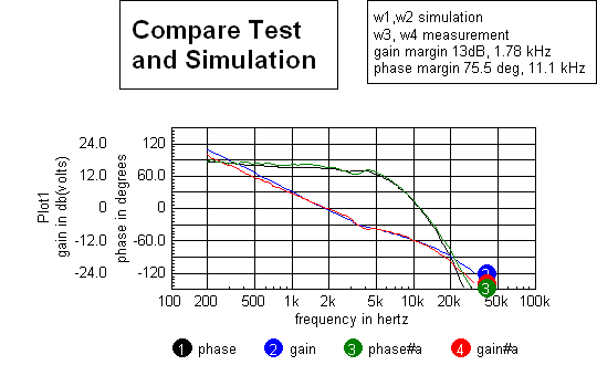
The hardware based AC analysis is a swept frequency transfer function analyzer based on single injection GFT theory. Running in about 20 seconds, it collects about 50 data points, from 200Hz to about .3*(Fs, the sampling frequency), as shown in the graphic to the right. The DSP generates a sine-cosine waveform algorithmically using much less memory than a table generated waveform generator. The cosine wave is scaled and inserted in series with the error signal. The coefficients for the waveform generator are transferred using RTCOM and the DSP waits for transient residues to stabilize, then it sums the product of cosine and sine times the signal. After 50ms of real time, it returns the result to IntuScope. IntuScope then computes the gain and phase for that frequency and advance to the next frequency. |
 |
|
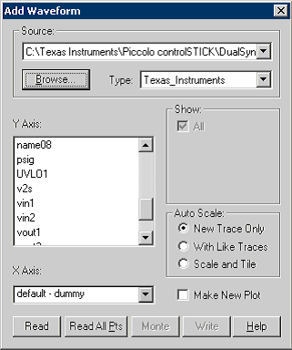
This corresponds to a SPICE DC operating point. It reads the steady state average of 1024 successive measurements of the specified vector. The IntuScope "Add Waveforms" dialog contains the standard 8-word interface along with user specified data and scaling. When SpiceNet drawing test points have the same name as the "Add Waveform" vectors, then SpiceNet can display the values by selecting "options/Stream DSP Testpoint Values" as shown in the graphic to the right. Averaging decreases noise by the square root of the number of samples; in this case, the virtual current estimate is 10ma RMS, which is equivalent to 8.7 bit accuracy. |
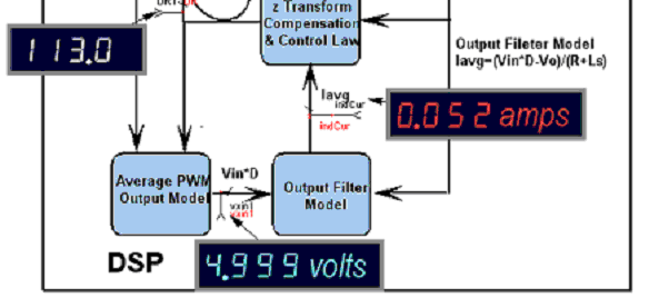 |
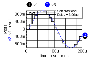
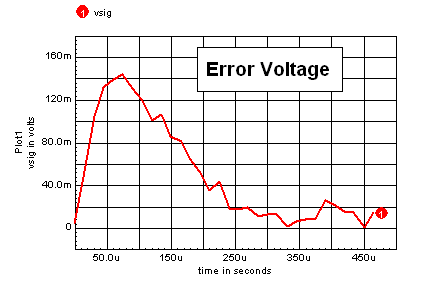
Lets you see the response of a named vector (from the "Add Waveforms" dialog) to a transient signal synchronized to TP5. TP5 drives an onboard MOSFET switch that can be connected externally to a load resistor. For each high-speed interrupt, one data point is added to the vector. Then the time slot in the vector for the data point is advanced by one sample. The built-in TRAN function takes 32 data points, averaged for 8 entire waveforms. It takes about 30 seconds to acquire the waveform. The internal error signal is plotted in the graphic to the right. This information is ONLY available in simulation or by using RTCOM because it is not available using hardware measurement because it is a mathematical representation inside of the DSP code. |
 |
|
_______________________Code
Generation_______________________
|
|
Schematic:
First, the user makes a schematic diagram of the controller in a separate
drawing configuration.
|
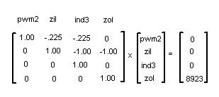
IsSpice4 Matrix:
Then, the ICAP/4 simulator builds a matrix that solves for the states
shown as nodes in the schematic. Parameters define the variables so that
the design becomes a template which applies to design variations
|
Sample of Assembly
Code: |
|
_______________
New ICAP/4 Models and Analysis________________
|
DSP controllers use
Z-Transforms to express a control law. Z-Transform transfer functions
can be mapped from the continuous or Laplace domain to the Z plane by
evaluation the defining equation:
Control expressions
can be written using the definition of integration and its inverse, differentiation
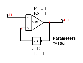
directly. The classical PID (proportional integral differential) controller
is a widely used example. It is one of the template designs included in
the DSP Designer projects. |
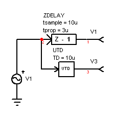
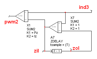
Typically, SPICE simulators
use the transmission line to model the unit delay |
The SPICE transient
simulation proceeds by solving a modified nodal admittance matrix, MNA.
It iterates the solution at each time point until its convergence criteria
is met. This method is required for solving non-linear equations. But
difference equations for a DSP controller can be made to be linear. Imposing
a linear constraint can result in an upper diagonal matrix (values below
the main diagonal are zero) that is used over and over for each DSP sample
time. If the matrix is ordered so that unwanted states are at the top
and trivial states at the bottom, then solution by backward substitution
from the fist non-trivial state to the first unwanted state produces a
solution in a single pass. Trivial states are identified as having just
one non-zero state in the matrix. For a linear matrix, the right hand
side, RHS, is zero for each non-trivial state. The new ".DSP"
analysis follows these rules. After the solution is made, the solution
for the ZDELAY inputs are propagated to their outputs before the next
sample, and are among the trivial states. Other trivial states are measured
inputs and outputs from other control algorithms. The resulting matrix
can be seen in the ".out" file. |