![]()
|
|
|
|
|
|
|
|
|
|
Intusoft’s software tools are widely used to synthesize and analyze power supplies. Over time, an increased feature set has made these tools more difficult to use because of the many ways the features can be combined to produce an acceptable design. To simplify the software use, we have introduced a comprehensive end-end design method for switch mode DC-DC converters. The framework consists of: |
|
||||||||||||||
|
Starting
with the Magnetics Designer, MD, using the Switch Mode Power Supply wizards;
the user enters the power supply specification and MD computes the Transformer
or Inductor spreadsheet entries. Data needed are input power supply voltage
and the output voltage(s) and current(s) along with frequency, duty ratio
and ripple current. An automatic design phase synthesizes the transformer/inductor. The user can then interact with MD to perfect the design. When acceptable results are achieved, an IsSpice model is generated for use in one of the template power supplies. The demo version produces designs with limited number of winding and core selection that are compatible with the ICAP/4 demo. A number of working power supply designs have been placed in a template framework. These templates include Flyback, Forward and Push-Pull topologies. The demo software will run average and switching models for these pre-designed templates. These templates accept the IsSpice transformer models generated using Magnetics Designer for cycle by cycle switching simulations. The transformer parameters can be input to the "Average" models. New "Average" models for Forward and Flyback work for both large and small signals with auto CCM/DCM switching and account for transport delay using a first order hold and Z-transform integrator. There are 2 classes of models, in the demo they are FORWARD_ID, and FLYBACK_ID and in the professional additional capabilities are included in the FORWARD_I and FLYBACK_I. These professional versions have resistive switching losses and dynamic switching losses modeled. They give a reasonable estimate of power supply efficiency just from the OP analysis. Included are objective functions for optimization of transient response and selection of input filter damping. Again, the optimizer can be run using the demo software. Intusoft’s new VSECTOL option has been set in the transient simulations to yield improved accuracy using fewer iterations than can be obtained with traditional Spice time step control methods. A built-in optimizer aids the designer in selecting critical control system parameters. It gets the most out of a design topology; frequently saving extra parts by getting the right transient wave shapes using the optimized component values. See http://www.intusoft.com/articles/PwrTemplate.pdf for an example and instructions on using the optimizer for power supply design. |
|
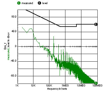
Both MIL-STD-462 and the EU CISPR16 line stabilization networks are used in the template power supplies to provide a test signal that’s used by the Scope5 waveform viewer to plot the EMI spectrum shown in Figure 1 along with the specification limits -- all at the press of one button. And there’s the one button Bode Plot available introduced in Newsletter 59 pp2-5. Here’s how it looks today.
|
|
|
Let’s run
through a sample design for a 5VDC off-line Flyback SMPS (Switch Mode
Power Supply). First; fire up Magnetics Designer, MD. Select the Inductor
tab. That’s right; a Flyback "transformer" is really an inductor
with the primary and secondary conducting at different times. See the
SMPS button in the inductor tab, just press it and move into the world
of DC-DC converters. |
|
In the past the MD data entry was difficult to compute because it’s up to the user to specify inductance, DC current, AC current, maximum current and Volt-second capacity. These parameters decouple the inductor design from application specific waveform shapes, but it requires quite a bit of pencil and paper or finger and keyboard calculation. We initialize the core family to one suitable for SMPS design. There are many more, including pot cores, planar cores and many other Ferrite geometries, different vendors and materials. What you need to input is your choice of frequency, duty ratio and percent ripple. The percent ripple is the pk-pk ripple with respect to the peak current. At 100% the power supply slips into discontinuous mode and you can select a smaller secondary duty ratio. DCM operation is pretty stressful so that you should use it only for low power designs. Making different designs with varying ripple and duty ratio lets you trade off DC stress (small AC ripple) vs. AC stress (high AC ripple). There is probably an optimum value over the range of 0 to 100% Iripple ; however, it will depend on your tolerance for things like Litz wire, multiple strands and foil wire. Our power supply will run with rectified DC from USA or EU power. Typically the DC voltage will be 150 or 300. Now the question is, what to use for the design point? In our experience, the best design comes from the lower voltage (higher current) specification, so we’ll enter 150 for the winding 1 voltage and press the Insert button to get a new winding for data entry. The voltage should include the rectifier drop so we’ll input 5.5 for the DC voltage and 10 for the current. The efficiency
includes transformer and switching losses. That’s it, unless you want
more outputs. Press the Apply button and MD will run through an automated
design picking the smallest core which keeps the estimated temperature
rise below the maximum rise (50 Deg C is the default). Here’s the result
after tweaking the design using techniques discussed in the MD documentation
in |
|
Figure 4. Bobbin tab shows the final design. |
|
Predicted loss is 1.1 watts at 300 Volt input and 1.3 watts for the 150 Volts input. The leakage inductance is 2.7 micro henries, all done using Heavy Formvar wire. The resulting IsSpice model can be either copied and pasted into the template drawing or saved in the parts library. Designs using Litz wire can withstand more ripple and operate at higher frequencies producing smaller magnetic components; however, Litz wire is more difficult to use and is more expensive. That’s an economic and perhaps an electro-political decision you must make. The gap field causes eddy current losses in the wire near the gap. Moving the wire at least 3 gap lengths away from the gap, using Litz wire, moving the gap or breaking the gap up into many small pieces can reduce this loss. In the limit, a distributed gap ferrite; for example kool mu, will not have any gap loss. These properties are all predicted using Magnetics Designer. The inductance, turns ratio and leakage inductance are all parameters used in the average models. These values are in the IsSpice model. The user needs to re-scale the template part values based on the frequency and power levels. Once that is done, the control system can be designed, first making it stable using the average model AC analysis and Bode Plots, then refine the values using the average models transient analysis and optimizer. |
|
Figure 5. Scope5 uses parametric cursors for load-lines. |
Finally the transient switching model can be
run to validate the average model results and measure dynamic power transistor
stress as shown in Figure 5. Then, the snubbers component values
can be optimized and EMI tests can be run to iterate the design further
to gain compliance. |
Each of these has one or more corresponding template drawings. Each template drawing has a transient switching configuration and an average model. Some of the template drawings also have hierarchical sub- drawings for the average and switching models that facilitate model development. |
|
|
3. Making custom
calculator entries: Look at the !User folder in <IcapsDir>\in\scripts.
All you have to do is make a text file with a ".scp" extension
in this folder or any other folder within the "Scripts" folder
and the script file will be immediately available for you in the Scope5
Calculator menu. By adding a 16 wide by 15 high bitmap with the same base
name, you can insert it in the toolbar to make a one button script. |
|
During
the model testing in Spicemod5, we noticed that the simulated TR and TS
values did not match the values entered into Spicemod5 for certain Darlington
transistors. For example, if a ZTX614 NPN macro model created in Spicemod5,
described in Figure 6, was run in the DarlNPN.DWG test schematic, we would
get the measurements of TS=3.030u and TR=281.3n. Compared with the Spicemod5
default values, TS = 2.8u and TR=615n; the SPICE simulated measurements
were about 8.21% and 54.2% off from the desired TS and TR respectively.
Our software modeling guru told us that it’s nearly impossible to make
an exact solution and that some kind of iteration using IsSpice was almost
certainly required. |
|
Figure 6. ZTX614 NPN Model created in Spicemod5. |
|
Figure 7. sm_DarlNPN netlist modification. |
The newly added ICAP/4 Window optimizer will help us to obtain the exact TR and TS values desired in the simulator. Since TS and TR values measured are determined by the TF and TR parameters specified in the QPWR NPN model, we have modified the sm_DarlNPN netlist, as shown in Figure 7, to pass the TF and TR parameters to the schematic level, because only schematic level parameters can be optimized. |
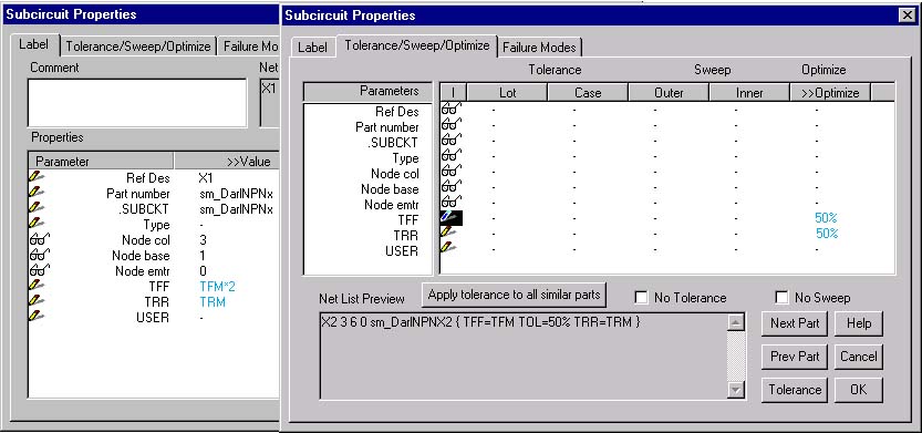
| These changes set the model parameters, TF and TR, to TFF and TRR. Two new parameters, TFM and TRM, were created in the params.txt file for initializing the TFF and TRR values during the optimization. TFM*2 and TRM were chosen to be the initial values for TFF and TRR, and 50% optimizing percentage was used for both TFF and TRR under the Tolerance/Sweep/ Optimize tab in the Subcircuit Properties dialog. This is illustrated in Figure 8. |
Figure 8. Initial values and optimizing percentage. |
|
The initial values and optimizing percentage are adjustable, depending on the optimization goal. Furthermore, an objective function was defined by using the script shown in Figure 9. The optimize script was modified to do three passes using a 3rd order polynomial with 7 data points. By running the opitimizer3rd three times, objective function and the optimized TRM and TFM values were obtained. The objective function should be close to 0. Replacing the TRM and TFM*2 with the bestval ( optimized TRM and TFM values ) in the Subcircuit Properties dialog would achieve the goal of having the TR and TS values to match the desired values. |
Figure 9. Script for the Optimizer Objective Function. |
|
MOS IC technology has made tremendous progress in recent years. The ever-increasing trend toward low-voltage and low-power deep submicron CMOS design has created a need for a more physical and compact MOS model. A clear understanding of the MOS transistor operation at very low current and a correct modeling in the weak and moderate inversion regions, which have been ignored by many designers and model builders for years, have become even more important issues for cost-effective design of high-performance analog and digital integrated circuits. Invented at EPFL in Lausanne Switzerland, the EKV MOSFET model is a scalable and compact simulation model built on fundamental physical properties of the MOS structure. This model is dedicated to the design and simulation of low-voltage, low-current analog, and mixed analog-digital circuits using submicron CMOS technologies. Its physical basis ensures excellent modeling of weak-to- strong inversion behavior for current, transconductances and gm/Id ratio. Due to the model’s increased availability in circuit simulators the EKV model is a powerful design tool, giving the designer insight into device and circuit operation and allowing faster design cycles. The EKV MOSFET model is in principle formulated as a ‘single expression’, which preserves continuity of first-and higher-order derivatives with respect to any terminal voltage, in the entire range of validity of the model. The EKV MOSFET model version 2.6 has been recently implemented in IsSpice as MOS model level 9. The following physical effects are included in this model: |
|
|
Here are a few more new scripts you’ll find in Scope5.
You can make your own scripts by following the format below and placing
them in a ".scp" file in the ...in\scripts subfolders. The scripts
subfolders are the same as the hierarchy shown in the calculator menu.
The first line is a comment line that will be displayed in the help status
at the bottom of the main window. The character following the optional
‘&’ symbol is the hotkey. If you create a bitmap (15 hi by 16 wide),
naming it with the same name as your script but with a .bmp extension,
you can make it a toolbar button using the options menu customize toolbar
dialog. You can also add a .htm file to provide further information about
your script. |
!User/expandx: |
|
This one illustrates the simplicity and power of the script language.
You place the cursors somewhere on the waveform and press x. The plot’s
x-axis is zoomed in to the region between the cursors.
|
!User/expandy: |
|
Similary to expand x except it makes the y-axis scaling for the selected
waveform full scale.
|
Functions/matchscales: |
|
Makes the y-axis scales of all waveforms the same as the current (selected) waveform. Notice how the hotkey combination works (x Y y) to expand and link scales in both x and y axis.
|
User/frequency: |
|
The latest release also includes the askvalues command, that prompts for user entry, see http://www.intusoft.com/script/pages/commands.htm#askvalues, for details.
|
|
Smith charts and TouchStone file reader along with
scripts for easy management of these data.
A new "append" command will be added to the ICL. It concatenates vectors and it will be used in a "superscript" function in Scope5 that collects all vectors in a plot into a single family. That’s useful in managing alter dialog sweeps and plot-all results. And finally; SpiceNet gets rubber banding. This was delayed
because of the added complexity caused by having to consider what to do
with parts on other layers not belonging to the configuration being edited.
We decided to move them also if there were any layers common to both configurations. |